When the response variable represent counts of some event, we usually model using the (log) rate with Poisson regression
Compares rates of response per space-time (e.g. person-years) across groups
“Rate ratio”
Why not use linear regression? The reasons are primarily statistical
The rate is in fact a mean
For Poisson \(Y\) having event rate \(\lambda\) measured over time \(t\)
The mean is equal to the variance (both are \(\lambda t\))
We want to be able to account for
Different areas of space or length of time for measuring counts
Mean-variance relationship (if not using robust standard errors)
In Poisson regression, we tend to use a log link when modeling the event rate
As in other models, a log link means that we are assuming a multiplicative modeling
Multiplicative model \(\rightarrow\) comparisons between groups based on ratios
Additive model \(\rightarrow\) comparisons between groups based on differences
Log link also has the best technical statistical properties
Log rate is the “canonical parameter” for the Poisson distribution
Being the canonical parameter makes the calculus and mathematical properties easier to derive, and thus easier to understand from a theoretical perspective
Poisson regression
Response variable is count of event over space-time (often person-years)
Offset variable specifies amount of space-time
Allows continuous or multiple grouping variables
But will also work with binary grouping variables
Simple Poisson Regression
Modeling rate of count response \(Y\) on predictor \(X\)
Rate when the predictor is \(0\) is found by exponentiation of the intercept from Poisson regression: \(e^{\beta_0}\)
Slope
Rate ratio between groups differing in the value of the predictor by 1 unit is found by exponentiation of the slope from Poisson regression: \(e^{\beta_1}\)
3 Example: Acid reflux and BMI
3.1 Data description
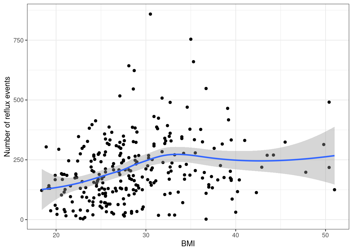
Research question: Are the number of acid reflux events in a day related to body mass index (BMI)?
Each subject pH in the esophagus in monitored continuously for about 24 hours
Count the number of time pH drop below 4, which is called a “reflux event”
Analysis (statistical) goals
Primary goal: Determine if there is an association between BMI and acid reflux rate
Secondary goal: Describe the (mean) trend in reflux rates as a function of BMI
Variables
Response: Number of acid reflux events
Offset: Number of minutes subject was monitored
Predictor of interest: BMI
Other covariates: Presence of esophagitis at baseline
3.2 Descriptive Plots
Code
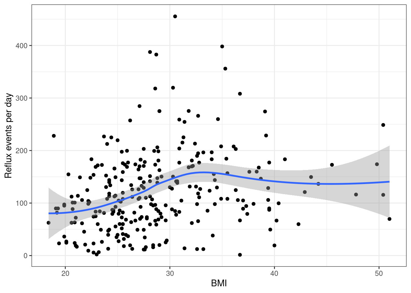
bmi.data <-read.csv("data/bmi.csv", header=TRUE)# Events are pH less than 4bmi.data$events <- bmi.data$totalmins4ggplot(bmi.data, aes(x=bmi, y=events)) +geom_point() +geom_smooth() +theme_bw() +xlab("BMI") +ylab("Number of reflux events")
Estimated event rate when BMI is 0 is found by exponentiation: \(e^{-3.12} = 0.044\)
This is the rate per 2-minute interval. This unusual time interval is an artifact of the way in pH data is sampled
To convert to events per day, multiply by 720 (there are 720 2-minute intervals in a day)
\(720 \times e^{-3.12} = 31.7 \textrm{ events per day}\)
Interpretation of slope
Estimated ratio of rates for two subjects differing by 1 in their BMI
Interpretation by exponentiation of slope
A subject with a 1 \(\textrm{kg} / m^2\) higher BMI will have an acid reflux event rate that is \(2.3\%\) higher. (calc: \(e^{0.0223} = 1.023\))
We are 95% confident that the increase in event rate is between \(1.3\%\) higher and \(3.2\%\) higher
There is a significant association between BMI and reflux events \(p < 0.001\)
4 Example: Acid reflux and BMI by esophagitis status
4.1 BMI modeled as a linear term
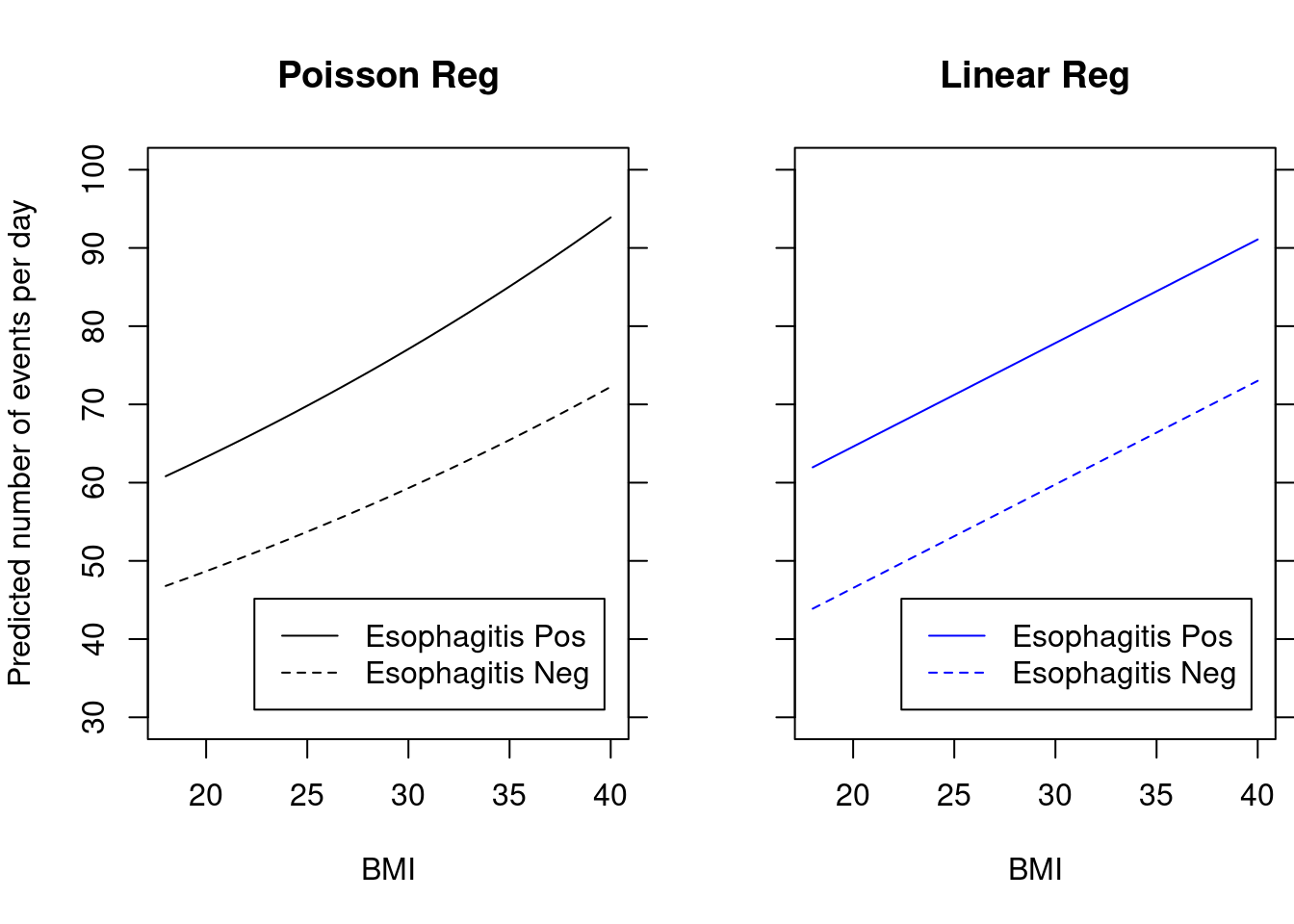
The following results compare using a Poisson model to a linear regression model
Both models will control for Esophagitis status, so any interpretation must involve “Holding esophagitis status constant…” (“Among subjects with the same Esophagitis status…”)
Note the different (numerical) estimates for the coefficients and standard errors for BMI and esophagitis, but the similar statistical significance
Also if we plot the predicted number of events per day versus BMI, the results are similar from either model
4.1.1 R: Poisson regression of events with offset for log(total time monitored)
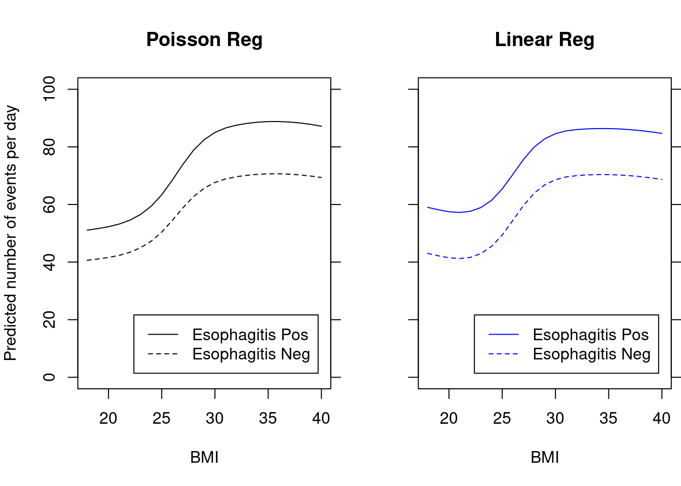
4.3 Comparison of modeling linear BMI to using spline function
For all regression models, we are more confident modeling associations than predicting means
When we use a linear term (i.e. a straight line) for the predictor, we are modeling a first-order association
Most power to detect this type of association
Always need to check that a first-order association answers the scientific question
Counter example: Interested in seasonal trends in air pollution. A linear effect of time would only answer if air pollution levels are increasing/decreasing over time, not how they are changing from month to month
Flexible functions for predictors, including splines, are, in general, more useful if we care about predicting means or individual observations
Acid reflux example: Which model you choose depends on the scientific goals
Primary goal: Is there an association between BMI and the rate of acid reflux?
Fitting the linear BMI term answers this question
Secondary goal: Describe the (mean) trend in reflux rates as a function of BMI
A priori, I would be less inclined to believe a linear function captures the true mean relationship
To answer this scientific question, a spline analysis is preferred
4.4 Bayesian Poisson Regression
4.4.1 Likelihood Function
The Bayesian analysis begins by specifying the likelihood and prior distributions.
For the Poisson model, the likelihood function can bewritten as:
where \(y_i\) is the observed count for each observation \(i\), and \(\lambda_i\) is the expected count.
In a Poisson regression model, \(\lambda\) is modeled as a function of the covariates X and coefficients \(\boldsymbol{\beta}\), such that:
\[\lambda = \exp(\textbf{X} \boldsymbol{\beta})\]
This equation links the expected counts to the linear predictor, allowing for the estimation of the effects of the covariates on the response variable.
(With the Poisson likelihood, we are still assuming the mean is equal to the variance)
4.4.2 Prior specification
As with any Bayesian analysis, prior distributions must be specified for all parameters in the model
For the Poisson regression model, \(\boldsymbol{\theta} = \boldsymbol{\beta}\)
A convenient choice of prior distribution for \(\boldsymbol{\beta}\) is the Multivariable Normal distribution
Here, \(\boldsymbol{\mu}\) represents the mean vector of the prior distribution, and \(\boldsymbol{\Sigma}\) represents the covariance matrix.
The prior mean \(\boldsymbol{\mu}\) and covariance \(\boldsymbol{\Sigma}\) can be chosen based on prior knowledge or elicited from experts, or can be set to non-informative values for a more objective analysis.
4.4.3 Posterior Distribution
The posterior distribution of \(\boldsymbol{\beta}\) is proportional to the product of the likelihood function and the prior distribution:
Where \(\lambda_i = \exp(\textbf{x}_i \cdot \boldsymbol{\beta})\), and \(p\) is the number of regression coefficients.
The posterior distribution is typically complex and does not have a closed-form expression, requiring numerical methods such as Markov chain Monte Carlo (MCMC) for inference.
In this course, we have been using rstanarm and stan_glm to perform MCMC
4.5 Bayesian Poisson regression example
To fit a Bayesian Poisson regression model using the rstanarm package, we can use the stan_glm() function.
The following code specifies a Bayesian model that is equivalent to the earlier frequentist model with bmi and esop and an offset
The mean_ppd is the sample average posterior predictive distribution of the outcome variable.
MCMC diagnostics
mcse
Rhat
n_eff
(Intercept)
0.00032
0.99956
3585
bmi
0.00001
0.99928
4015
esop
0.00027
1.00178
1503
mean_PPD
0.02521
1.00112
2267
log-posterior
0.03244
1.00201
1334
For each parameter, mcse is Monte Carlo standard error, n_eff is a crude measure of effective sample size, and Rhat is the potential scale reduction factor on split chains (at convergence Rhat=1).
In this code:
events ~ bmi + esop + offset(log(totalmins)) specifies the model formula.
family = poisson(link = "log") specifies a Poisson distribution with a log link function
prior = normal(location = 0, scale = 1) and prior_intercept = normal(location = 0, scale = 1) specify priors for the regression coefficients and intercept.
seed = 1234 sets a random seed to ensure reproducibility of the results.
refresh = 0 suppresses the progress bar during model fitting.
And a summary of the prior distributions used
Code
prior_summary(m2.bayes.poisson, digits =2)
Priors for model ‘m2.bayes.poisson’
Specified prior
Adjusted prior
Intercept (after predictors centered)
~ normal(location = 0, scale = 1.00000)
Coefficients
~ normal(location = 0, scale = 1.00000)
~ normal(location = 0, scale = 1.00000)
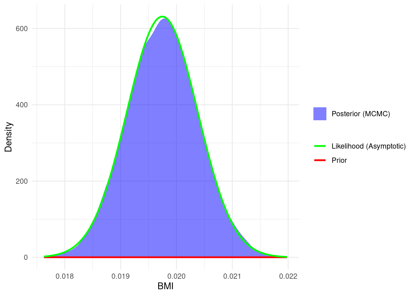
4.5.1 Plot of Prior, Likelihood, Posterior
The following shows the prior, likelihood and the posterior for the Poisson model of the \(\beta\) for BMI.
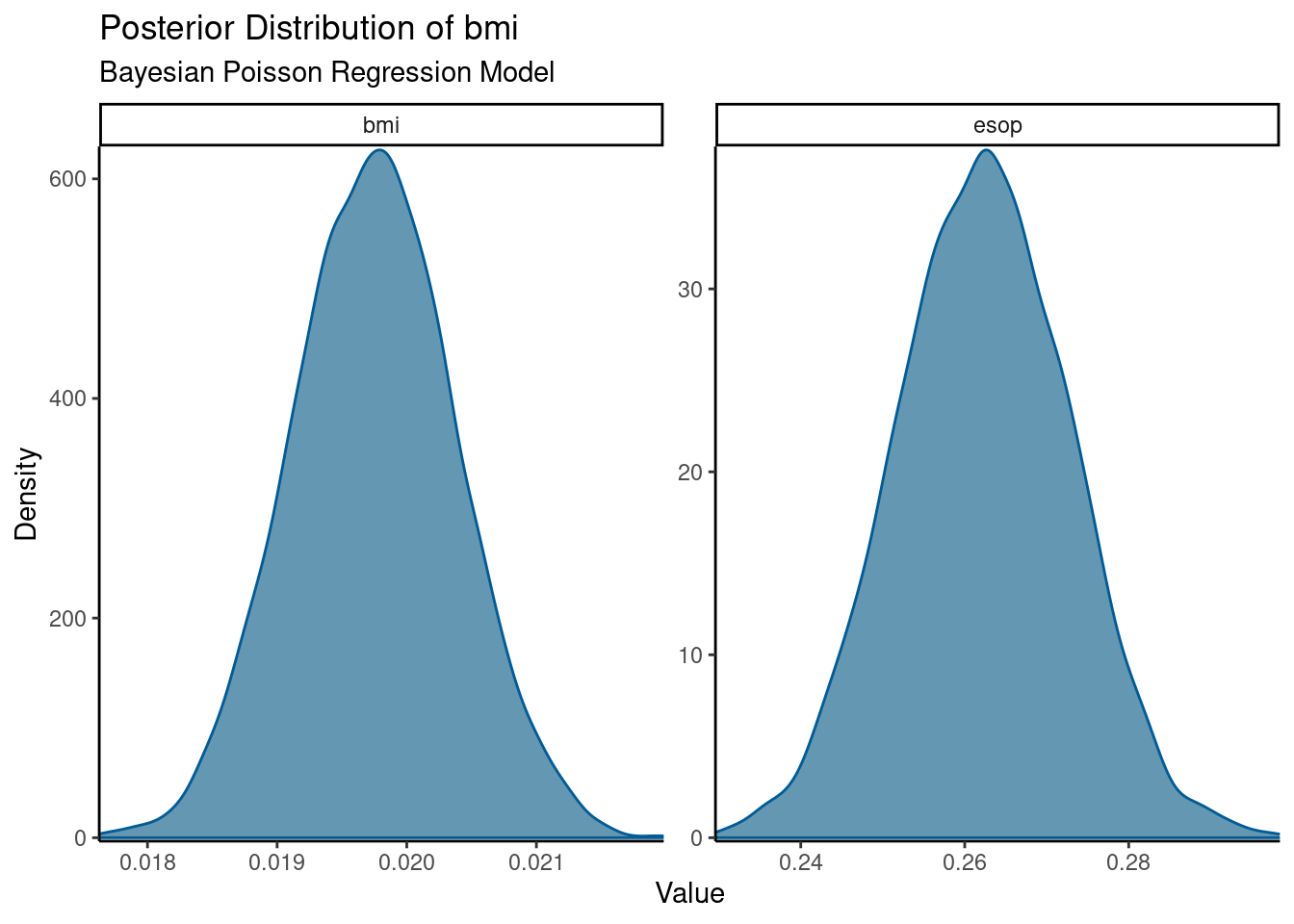
Here is just the posterior distributions for BMI and esop
Code
library(bayesplot)mcmc_dens(m2.bayes.poisson, pars=c("bmi","esop")) +labs(title ="Posterior Distribution of bmi",subtitle ="Bayesian Poisson Regression Model",x ="Value", y ="Density") +theme_classic()
---title: "Poisson Regression"subtitle: "Lecture 09"name: Lec09.Poisson.qmd---```{r}#| echo: falselibrary(rms)library(ggplot2)library(splines)tryCatch(source('pander_registry.R'), error =function(e) invisible(e))```## Count Data and Event Rates- Sometimes a random variable measures the number of events occurring over some space and time interval- Examples include - Number of polyps recurring in the three year interval between colonoscopies - Number of pulmonary exacerbations experienced by a cystic fibrosis patient in a year - Number of reflux events in a 24-hour period- Count data have (in theory) no upper limit, although very large counts can be highly improbable- When a response variable measures counts over space and time, we often summarize by considering the event rate - "Event rate" is the expected number of events per unit of space-time - The rate is thus a mean count - In most statistical problems, we know the interval of time and the volume of space sampled - Poisson models allow us to take into account the known interval of time/space using an "offset"## Poisson Model### Poisson distribution- Often we assume that counts follow a Poisson distribution- The Poisson distribution can be derived from the following assumptions - The expected number of events in an interval is proportional to the size of the interval - The probability that two events occur with an infinitesimally small interval of space-time is zero - The number of events occurring in disjoint (separate) intervals of space-time are independent- (Note that the assumption of a constant rate with independence over space-time is pretty strong and rarely holds completely)- Poisson distribution - Counts the events occurring at a constant rate $\lambda$ in a specified time (and space) $t$ - Independent intervals of time and space - Probability distribution has parameter $\lambda > 0$ - For $k = 0, 1, 2, \ldots$ $$\textrm{Pr}(Y = k) = \frac{e^{-\lambda t} (\lambda t)^k}{k!}$$ - Mean: $E[Y] = \lambda t$ - Var: $V[Y] = \lambda t$ - (Mean-variance relationship, like binary data)### Regression Model- When the response variable represent counts of some event, we usually model using the (log) rate with Poisson regression - Compares rates of response per space-time (e.g. person-years) across groups - "Rate ratio"- Why not use linear regression? The reasons are primarily statistical - The rate is in fact a mean - For Poisson $Y$ having event rate $\lambda$ measured over time $t$ - The mean is equal to the variance (both are $\lambda t$) - We want to be able to account for - Different areas of space or length of time for measuring counts - Mean-variance relationship (if not using robust standard errors)- In Poisson regression, we tend to use a log link when modeling the event rate - As in other models, a log link means that we are assuming a multiplicative modeling - Multiplicative model $\rightarrow$ comparisons between groups based on ratios - Additive model $\rightarrow$ comparisons between groups based on differences - Log link also has the best technical statistical properties - Log rate is the "canonical parameter" for the Poisson distribution - Being the canonical parameter makes the calculus and mathematical properties easier to derive, and thus easier to understand from a theoretical perspective- Poisson regression - Response variable is count of event over space-time (often person-years) - Offset variable specifies amount of space-time - Allows continuous or multiple grouping variables - But will also work with binary grouping variables- Simple Poisson Regression - Modeling rate of count response $Y$ on predictor $X$ - Distribution: $\textrm{Pr}(Y_i = k | T_i = t_i) = \frac{e^{-\lambda_i t_i} (\lambda_i t_i)^k}{k!}$ - Model: $\textrm{log } E[Y_i | T_i, X_i] = \textrm{log}\left(\lambda_i T_i\right) = \textrm{log}(T_i) + \beta_0 + \beta_1 \times X_i$ - $X_i = 0$: log $\lambda_i = \beta_0$ - $X_i = x$: log $\lambda_i = \beta_0 + \beta_1 \times x$ - $X_i = x+1$: log $\lambda_i = \beta_0 + \beta_1 \times x + \beta_1$ - To interpret as rates, exponentiate the parameters - Distribution: $\textrm{Pr}(Y_i = k | T_i = t_i) = \frac{e^{-\lambda_i t_i} (\lambda_i t_i)^k}{k!}$ - Model: $\textrm{log } E[Y_i | T_i, X_i] = \textrm{log}\left(\lambda_i T_i\right) = \textrm{log}(T_i) + \beta_0 + \beta_1 \times X_i$ - $X_i = 0$: $\lambda_i = e^{\beta_0}$ - $X_i = x$: $\lambda_i = e^{\beta_0 + \beta_1 \times x}$ - $X_i = x+1$: $\lambda_i = e^{\beta_0 + \beta_1 \times x + \beta_1}$- Interpretation of the model - Intercept - Rate when the predictor is $0$ is found by exponentiation of the intercept from Poisson regression: $e^{\beta_0}$ - Slope - Rate ratio between groups differing in the value of the predictor by 1 unit is found by exponentiation of the slope from Poisson regression: $e^{\beta_1}$## Example: Acid reflux and BMI### Data description- Research question: Are the number of acid reflux events in a day related to body mass index (BMI)?- Each subject pH in the esophagus in monitored continuously for about 24 hours- Count the number of time pH drop below 4, which is called a "reflux event"- Analysis (statistical) goals - Primary goal: Determine if there is an association between BMI and acid reflux rate - Secondary goal: Describe the (mean) trend in reflux rates as a function of BMI- Variables - Response: Number of acid reflux events - Offset: Number of minutes subject was monitored - Predictor of interest: BMI - Other covariates: Presence of esophagitis at baseline### Descriptive Plots```{r, fig.cap="BMI by number of reflux events"}bmi.data <-read.csv("data/bmi.csv", header=TRUE)# Events are pH less than 4bmi.data$events <- bmi.data$totalmins4ggplot(bmi.data, aes(x=bmi, y=events)) +geom_point() +geom_smooth() +theme_bw() +xlab("BMI") +ylab("Number of reflux events")``````{r, fig.cap="BMI by number of reflux events per day"}bmi.data$rate <- bmi.data$totalmins4/bmi.data$totalmins*60*24ggplot(bmi.data, aes(x=bmi, y=rate)) +geom_point() +geom_smooth() +theme_bw() +xlab("BMI") +ylab("Reflux events per day")```- Characterization of plots - Plots are visually similar if we consider the rate (events per day) or the raw number of events - First order trend: Event rate increases with increasing BMI - Second order trend: Event rate increase until BMI of 32 (or so) and then flattens out - Within-group variability - Hard to visualize from the plots - Model assumes increasing variability with increasing BMI, which looks reasonable### Regression commands- As before, but need to specify the offset - Offset is the log of the exposure time - In Stata, can alternatively specify the "exposure" and it will take the log for you- Stata - `poisson respvar predvar, exposure(time) [robust]` - `poisson respvar predvar, offset(logtime) [robust]`- R - One method to fit Poisson models - Uses the `sandwich` and `lmtest` libraries - Must install the above two libraries using `install.packages("lmtest")` and `install.packages("sandwich")` - `model.poisson <- glm(response ~ predictors + offset(log(time)), data=data, family="poisson")` - `coeftest(model.poisson, vcov=sandwich)` - Another method to fit Poisson models using the `Design` package - `m1 <- glmD(response ~ predictors + offset(log(time)), data=data, family="poisson", x=TRUE, y=TRUE)` - `bootcov(m1)` for robust (bootstrap) confidence intervals - Can also use methods within the `gee` library### Estimation of the regression model- Regression model for number of reflux events on BMI - Answer primary research question: Is there an *association* between BMI and the acid reflux event rate? - Estimate the best fitting line to (log) number of reflux events within BMI groups using an offset of log time - $\textrm{log}(\textrm{Events} | \textrm{BMI}) = \beta_0 + \beta_1 \times \textrm{BMI} + \textrm{log}(\textrm{time})$ - An association will exist if the slope $\beta_1$ is nonzero```{r}library(lmtest)library(sandwich)m1.poisson <-glm(events ~ bmi +offset(log(totalmins)), data=bmi.data, family="poisson")m1.poissoncoeftest(m1.poisson, vcov=sandwich)confint(coeftest(m1.poisson, vcov=sandwich))`````` stata. poisson events bmi, offset(logmins) robustIteration 0: log pseudolikelihood = -11360.89 Iteration 1: log pseudolikelihood = -11360.89 Poisson regression Number of obs = 279 Wald chi2(1) = 23.42 Prob > chi2 = 0.0000Log pseudolikelihood = -11360.89 Pseudo R2 = 0.0520------------------------------------------------------------------------------ | Robust events | Coef. Std. Err. z P>|z| [95% Conf. Interval]-------------+---------------------------------------------------------------- bmi | .0223194 .0046121 4.84 0.000 .0132799 .0313589 _cons | -3.119991 .139521 -22.36 0.000 -3.393448 -2.846535 logmins | (offset)------------------------------------------------------------------------------```- Interpretation of output - $\textrm{log rate} = -3.119991 + 0.0223194 \times \textrm{BMI}$- Interpretation of intercept - Estimated event rate when BMI is 0 is found by exponentiation: $e^{-3.12} = 0.044$ - This is the rate per 2-minute interval. This unusual time interval is an artifact of the way in pH data is sampled - To convert to events per day, multiply by 720 (there are 720 2-minute intervals in a day) - $720 \times e^{-3.12} = 31.7 \textrm{ events per day}$- Interpretation of slope - Estimated ratio of rates for two subjects differing by 1 in their BMI - Interpretation by exponentiation of slope - A subject with a 1 $\textrm{kg} / m^2$ higher BMI will have an acid reflux event rate that is $2.3\%$ higher. (calc: $e^{0.0223} = 1.023$) - We are 95% confident that the increase in event rate is between $1.3\%$ higher and $3.2\%$ higher - There is a significant association between BMI and reflux events $p < 0.001$## Example: Acid reflux and BMI by esophagitis status### BMI modeled as a linear term- The following results compare using a Poisson model to a linear regression model- Both models will control for Esophagitis status, so any interpretation must involve "Holding esophagitis status constant..." ("Among subjects with the same Esophagitis status...")- Note the different (numerical) estimates for the coefficients and standard errors for BMI and esophagitis, but the similar statistical significance- Also if we plot the predicted number of events per day versus BMI, the results are similar from either model#### R: Poisson regression of events with offset for log(total time monitored)```{r}m2.poisson <-glm(events ~ bmi + esop +offset(log(totalmins)), data=bmi.data, family="poisson")m2.poissoncoeftest(m2.poisson, vcov=sandwich)confint(coeftest(m2.poisson, vcov=sandwich))```#### R: Linear regression of rate (events/time) as outcome```{r}bmi.data$rate <- bmi.data$events / bmi.data$totalminsm2.lm <-lm(rate ~ bmi + esop, data=bmi.data)m2.lmcoeftest(m2.lm, vcov=sandwich)confint(coeftest(m2.lm, vcov=sandwich))```#### Stata Output``` stata. poisson events bmi esop, offset(logmins) robustPoisson regression Number of obs = 279 Wald chi2(2) = 30.30 Prob > chi2 = 0.0000Log pseudolikelihood = -11072.339 Pseudo R2 = 0.0761------------------------------------------------------------------------------ | Robust events | Coef. Std. Err. z P>|z| [95% Conf. Interval]-------------+---------------------------------------------------------------- bmi | .0197465 .0047721 4.14 0.000 .0103934 .0290997 esop | .2622171 .083202 3.15 0.002 .0991442 .42529 _cons | -3.089033 .1423038 -21.71 0.000 -3.367944 -2.810123 logmins | (offset)------------------------------------------------------------------------------. gen eventsmins = events / mins. regress eventsmins bmi esop, robustLinear regression Number of obs = 279 F( 2, 276) = 14.16 Prob > F = 0.0000 R-squared = 0.0856 Root MSE = .05102------------------------------------------------------------------------------ | Robust eventsmins | Coef. Std. Err. t P>|t| [95% Conf. Interval]-------------+---------------------------------------------------------------- bmi | .001839 .0004618 3.98 0.000 .0009299 .0027482 esop | .025104 .0085449 2.94 0.004 .0082826 .0419254 _cons | .0278461 .0129053 2.16 0.032 .0024407 .0532515------------------------------------------------------------------------------```#### Comparison of predicted number of events from linear regression and Poisson regression models- Example prediction calculations: BMI=30, with esophagitis - Linear regression: $0.0278461 + .025104 + .001839 \times 30 = 0.108$ - Stata: `adjust bmi=30 esop=1` - Poisson regression: $e^{-3.089033 + 0.2622171 + .01975465 \times 30} = 0.107$ - Stata: `adjust bmi=30 esop=1, nooffset exp` - Remember the above rates are for a 2-minute time interval. To convert to daily rates, multiply by 720```{r}# Predicted events per two minute time intervalpredict(m2.lm, newdata=data.frame(bmi=30,esop=1))exp(predict(m2.poisson, newdata=data.frame(bmi=30,esop=1,totalmins=1), type="link"))# Predicted events per day (720 2-minute time intervals per day)predict(m2.lm, newdata=data.frame(bmi=30,esop=1))*720exp(predict(m2.poisson, newdata=data.frame(bmi=30,esop=1,totalmins=720), type="link"))``````{r}bmi.data$esop.factor <-factor(bmi.data$esop, levels=0:1, labels=c("Esop Neg", "Esop Pos"))m.spline2.adj <-glm(events ~ bmi +offset(log(totalmins)) + esop, data=bmi.data, family="poisson")m.spline3.adj <-lm(events / totalmins ~ bmi + esop, data=bmi.data)par(mfrow=c(1,2), mar=c(5,4,4,0.5))plot(18:40, exp(predict(m.spline2.adj, newdata=data.frame(bmi=18:40, totalmins=720, esop=1), type="link")), type='l', ylab="Predicted number of events per day", xlab="BMI", ylim=c(30,100), main="Poisson Reg")axis(4, labels=FALSE, ticks=TRUE)legend("bottomright", c("Esophagitis Pos","Esophagitis Neg"), inset=0.05, col=1, lty=1:2)lines(18:40, exp(predict(m.spline2.adj, newdata=data.frame(bmi=18:40, totalmins=720, esop=0), type="link")), lty=2)plot(18:40, 720*predict(m.spline3.adj, newdata=data.frame(bmi=18:40, esop=1), type="response"), type='l', col='Blue', ylab="", xlab="BMI", ylim=c(30,100), main="Linear Reg", axes=FALSE)axis(1)axis(4)axis(2, labels=FALSE, ticks=TRUE)box()lines(18:40, 720*predict(m.spline3.adj, newdata=data.frame(bmi=18:40, esop=0), type="response"), type='l', col='Blue', lty=2)legend("bottomright", c("Esophagitis Pos","Esophagitis Neg"), inset=0.05, col="Blue", lty=1:2)```### BMI modeled using splines- Regression splines are handled more naturally in R than in Stata - `glm(events ~ ns(bmi,4) + esop + offset(log(totalmins)), data=bmi.data, family="poisson")` - `ns(bmi, 4)` specified a natural spline for bmi with 4 degrees of freedom- Note that there is an optical illusion in the following plots - For both plots, it appears as if the lines are closer in the middle ranges of BMI - For the Poisson regression, the true distance between lines is increasing with increasing with BMI - For the Linear regrression, the true distance between lines is constant```{r}m.spline2.adj <-glm(events ~ns(bmi,4) +offset(log(totalmins)) + esop, data=bmi.data, family="poisson")m.spline3.adj <-lm(events / totalmins ~ns(bmi,4) + esop, data=bmi.data)par(mfrow=c(1,2), mar=c(5,4,4,0.5))plot(18:40, exp(predict(m.spline2.adj, newdata=data.frame(bmi=18:40, totalmins=720, esop=1), type="link")), type='l', ylab="Predicted number of events per day", xlab="BMI", ylim=c(0,100), main="Poisson Reg")axis(4, labels=FALSE, ticks=TRUE)legend("bottomright", c("Esophagitis Pos","Esophagitis Neg"), inset=0.05, col=1, lty=1:2)lines(18:40, exp(predict(m.spline2.adj, newdata=data.frame(bmi=18:40, totalmins=720, esop=0), type="link")), lty=2)plot(18:40, 720*predict(m.spline3.adj, newdata=data.frame(bmi=18:40, esop=1), type="response"), type='l', col='Blue', ylab="", xlab="BMI", ylim=c(0,100), main="Linear Reg", axes=FALSE)axis(1)axis(4)axis(2, labels=FALSE, ticks=TRUE)box()lines(18:40, 720*predict(m.spline3.adj, newdata=data.frame(bmi=18:40, esop=0), type="response"), type='l', col='Blue', lty=2)legend("bottomright", c("Esophagitis Pos","Esophagitis Neg"), inset=0.05, col="Blue", lty=1:2)```### Comparison of modeling linear BMI to using spline function- For all regression models, we are more confident modeling associations than predicting means- When we use a linear term (i.e. a straight line) for the predictor, we are modeling a first-order association - Most power to detect this type of association - Always need to check that a first-order association answers the scientific question - Counter example: Interested in seasonal trends in air pollution. A linear effect of time would only answer if air pollution levels are increasing/decreasing over time, not how they are changing from month to month- Flexible functions for predictors, including splines, are, in general, more useful if we care about predicting means or individual observations- Acid reflux example: Which model you choose depends on the scientific goals - Primary goal: Is there an association between BMI and the rate of acid reflux? - Fitting the linear BMI term answers this question - Secondary goal: Describe the (mean) trend in reflux rates as a function of BMI - A priori, I would be less inclined to believe a linear function captures the true mean relationship - To answer this scientific question, a spline analysis is preferred### Bayesian Poisson Regression#### Likelihood Function- The Bayesian analysis begins by specifying the likelihood and prior distributions.- For the Poisson model, the likelihood function can bewritten as:$$L(y | \lambda) = \prod_{i=1}^{n} \frac{e^{-\lambda_i} \lambda_i^{y_i}}{y_i!}$$where $y_i$ is the observed count for each observation $i$, and $\lambda_i$ is the expected count.- In a Poisson regression model, $\lambda$ is modeled as a function of the covariates **X** and coefficients $\boldsymbol{\beta}$, such that:$$\lambda = \exp(\textbf{X} \boldsymbol{\beta})$$- This equation links the expected counts to the linear predictor, allowing for the estimation of the effects of the covariates on the response variable.- (With the Poisson likelihood, we are still assuming the mean is equal to the variance)#### Prior specification- As with any Bayesian analysis, prior distributions must be specified for all parameters in the model- For the Poisson regression model, $\boldsymbol{\theta} = \boldsymbol{\beta}$- A convenient choice of prior distribution for $\boldsymbol{\beta}$ is the Multivariable Normal distribution$$\pi(\boldsymbol{\beta}) \sim \mathcal{N}(\boldsymbol{\mu}, \boldsymbol{\Sigma})$$- Here, $\boldsymbol{\mu}$ represents the mean vector of the prior distribution, and $\boldsymbol{\Sigma}$ represents the covariance matrix.- The prior mean $\boldsymbol{\mu}$ and covariance $\boldsymbol{\Sigma}$ can be chosen based on prior knowledge or elicited from experts, or can be set to non-informative values for a more objective analysis.#### Posterior Distribution- The posterior distribution of $\boldsymbol{\beta}$ is proportional to the product of the likelihood function and the prior distribution:$$\pi(\boldsymbol{\beta} | \textbf{y}) \propto L(\textbf{y} | \lambda) \cdot f(\boldsymbol{\beta})$$- Substituting the Poisson likelihood and multivariate normal prior, we get:$$\pi(\boldsymbol{\beta} | \textbf{y}) \propto \prod_{i=1}^{n} \frac{e^{-\lambda_i} \lambda_i^{y_i}}{y_i!} \cdot \frac{1}{\sqrt{(2\pi)^p |\boldsymbol{\Sigma}|}} \exp\left(-\frac{1}{2} (\boldsymbol{\beta} - \boldsymbol{\mu})^T \boldsymbol{\Sigma}^{-1} (\boldsymbol{\beta} - \boldsymbol{\mu})\right)$$- Where $\lambda_i = \exp(\textbf{x}_i \cdot \boldsymbol{\beta})$, and $p$ is the number of regression coefficients.- The posterior distribution is typically complex and does not have a closed-form expression, requiring numerical methods such as Markov chain Monte Carlo (MCMC) for inference. - In this course, we have been using `rstanarm` and `stan_glm` to perform MCMC### Bayesian Poisson regression example* To fit a Bayesian Poisson regression model using the `rstanarm` package, we can use the `stan_glm()` function.* The following code specifies a Bayesian model that is equivalent to the earlier frequentist model with bmi and esop and an offset```{r}library(rstanarm)m2.bayes.poisson <-stan_glm( events ~ bmi + esop +offset(log(totalmins)),data = bmi.data,family =poisson(link ="log"),prior =normal(location =0, scale =1),prior_intercept =normal(location =0, scale =1),refresh=0,seed=12345)summary(m2.bayes.poisson, digits=4, prob=c(.025, .5, .975))```- In this code: - `events ~ bmi + esop + offset(log(totalmins))` specifies the model formula. - `family = poisson(link = "log")` specifies a Poisson distribution with a log link function - `prior = normal(location = 0, scale = 1)` and `prior_intercept = normal(location = 0, scale = 1)` specify priors for the regression coefficients and intercept. - `seed = 1234` sets a random seed to ensure reproducibility of the results. - `refresh = 0` suppresses the progress bar during model fitting.- And a summary of the prior distributions used```{r}prior_summary(m2.bayes.poisson, digits =2)```#### Plot of Prior, Likelihood, Posterior- The following shows the prior, likelihood and the posterior for the Poisson model of the $\beta$ for BMI.```{r}plp.plotdata <-data.frame(post.draws=as.matrix(m2.bayes.poisson)[,"bmi"])density_plot <-ggplot(plp.plotdata, aes(x = post.draws)) +geom_density(aes(fill ="Posterior (MCMC)"), color =NA, alpha =0.5) +labs(x ="BMI", y ="Density") +scale_fill_manual(values =c("Posterior (MCMC)"="blue")) +stat_function(fun = dnorm, args =list(mean =0.0, sd =1), aes(color ="Prior"), size=1) +scale_color_manual(name="Legend", values =c("Prior"="red", "Likelihood (Asymptotic)"="green")) +stat_function(fun = dnorm, args =list(mean =coef(m2.poisson)["bmi"], sd =sqrt(vcov(m2.poisson)["bmi","bmi"])), aes(color ="Likelihood (Asymptotic)"), size=1) +theme_minimal() +theme(legend.title=element_blank())print(density_plot)```- Here is just the posterior distributions for BMI and `esop````{r}library(bayesplot)mcmc_dens(m2.bayes.poisson, pars=c("bmi","esop")) +labs(title ="Posterior Distribution of bmi",subtitle ="Bayesian Poisson Regression Model",x ="Value", y ="Density") +theme_classic()``````{r}posterior_vs_prior(m2.bayes.poisson, pars=c("bmi","esop"))```* A comparison of the coefficients estimates from the frequentist and Bayesian approaches```{r}rbind(glm=coef(m2.poisson),Bayes.weak=coef(m2.bayes.poisson))```* And a comparsion of the estimated standard errors for the intercept and the slopes```{r}rbind(glm=sqrt(diag(vcov(m2.poisson))),glm.robust=sqrt(diag(sandwich(m2.poisson))),Bayes.weak=sqrt(diag(vcov(m2.bayes.poisson))))```* Note that the standard errors are quite different from the roubst approach* From descriptive statistics, the mean and variance are quite different. The standard Poisson model assumes the mean equals the variance.```{r}c(mean=mean(bmi.data$rate), var=var(bmi.data$rate))library(dplyr)bmi.data <- bmi.data %>%mutate(bmi_quartile =cut2(bmi, g =4))bmi.data %>%group_by(bmi_quartile, esop) %>%summarise(mean_rate =mean(rate, na.rm =TRUE), var_rate =var(rate, na.rm =TRUE))```