Precision of Statistical Intefence

Download Code

Lecture 05

Chris Slaughter

October 30, 2025

tryCatch(source('pander_registry.R'), error = function(e) invisible(e))

1 Overview

• Goal of statistical inference is to estimate parameters accurately (unbiased) and with high precision

• Measures of precision

  • Standard error (not standard deviation)

  • Width of confidence intervals

  • Power (equivalently, type II error rate)

• Scientific hypotheses are typically refined in statistical hypotheses by identifying some parameter, \(\theta\), measuring differences in the distribution of the response variable

• Often we are interested in if \(\theta\) differs across of levels of categorical (e.g. treatment/control) or continuous (e.g. age) predictor variables

• \(\theta\) could be any summary measure such as

  • Difference/ratio of means

  • Difference/ratio of medians

  • Ratio of geometric means

  • Difference/ratio of proportions

  • Odds ratio, relative risk, risk difference

  • Hazard ratio

• How to select \(\theta\)? In order of importance…

1. Scientific (clinical) importance. May be based on current state of knowledge

2. Is \(\theta\) likely to vary across the predictor of interest? Impacts the ability to detect a difference, if it exists.

3. Statistical precision. Only relevant if all other factors are equal.

• Statistics is concerned with making inference about population parameters, (\(\theta\)), based on a sample of data

  • Frequentist estimation includes both point estimates (\(\hat{\theta}\)) and interval estimates (confidence intervals)

  • Bayesian analysis estimates the posterior distribution of \(\theta\) given the sampled data, \(p(\theta | \textrm{data})\). The posterior distribution can then be summarized by quantities like the posterior mean and 95% credible interval.

1.1 Example

Consider the following results from 5 clinical trials of three drugs (A, B, C) designed to lower cholesterol compared to baseline. Assume a 10 unit drop in cholesterol (relative to baseline) is clinically meaningful.

Trial	Drug	Pts	Mean diff	Std dev	Std error	95% CI for diff	p-value
1	A	30	-30	191.7	49.5	[-129, 69]	0.55
2	A	1000	-30	223.6	10	[-49.6, -10.4]	0.002
3	B	40	-20	147.6	33	[-85, 45]	0.55
4	B	4000	-2	147.6	3.3	[-8.5, 4.5]	0.54
5	C	5000	-6	100.0	2	[-9.9, -2.1]	0.002

• Compare the results of the different trials with respect to the sample size, mean difference, etc.

  • Which drug is effective at reducing cholesterol?

  • Why is study 4 more informative than study 3 (even though the \(p\) values are similar)?

  • Key points

    • Hypothesis tests and \(p\)-values can often be insufficient to make proper decisions. The confidence interval provides more useful information.
    • Narrower confidence intervals (more precise estimates) allow for scientific conclusion regardless of the \(p\) value

2 Precision variables and regression modeling

2.1 Definition

• Pure precision variables are associated with the outcome only

  • That is, no association (in the sample) with the predictor of interest

• In a randomized trial where random treatment assignment is the predictor of interest it may be possible to have a pure precision variable by using stratified randomization

  • Stratified randomization can guarantee that there is no correlation between the precision variable and treatment group assignment

• In observational research, there may be some correlation between the precision variable and the predictor of interest

  • May act more like a confounder in these cases, depending on the size of the association

2.2 Directed Acyclic Graph

flowchart LR
  X[Predictor\nof interest] --> Y[Outcome]
  W[Precision] --> Y[Outcome]

2.3 Example

2.3.1 Data generation

• Categorical precision variable (W), Predictor of Interest (X), Outcome (Y)

# Generate some data
set.seed(1231)
n <- 200
precisiondata <- 
  data.frame(W=rep(0:1, each=n/2),
             X=runif(n),
             Y=NA
)
precisiondata$Y <- 10 + 1.5*precisiondata$X + 10*precisiondata$W + rnorm(n,0,4)
precisiondata$W <- factor(precisiondata$W)

2.3.2 Bivariate plots

• W is uncorrelated with X, and associated with Y

library(ggplot2)
ggplot(precisiondata, aes(x=W,y=X)) + geom_boxplot()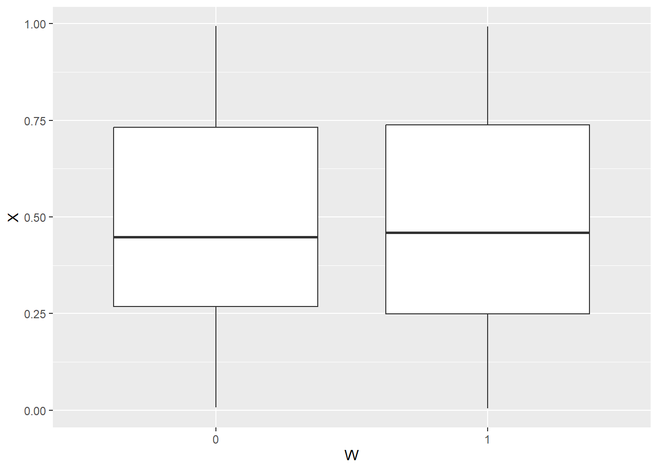

Box plot showing the (lack of) association between the precision variable (W) and the predictor of interest (X)

ggplot(precisiondata, aes(x=W,y=Y)) + geom_boxplot()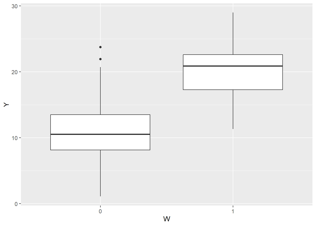

Box plot showing the association between the precision variable (W) and the outcome (Y)

ggplot(precisiondata, aes(x=X,y=Y)) + geom_point() + geom_smooth(method="lm")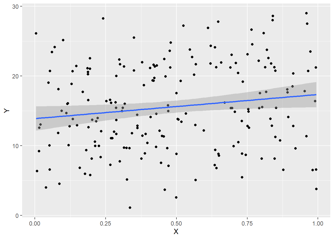

Association between the predictor of interest (X) and the outcome (Y) ignoring the precision variable (W)

2.3.3 Bivariate plot by W

ggplot(precisiondata, aes(x=X,y=Y,color=W,group=W)) + geom_point() + geom_smooth(method="lm")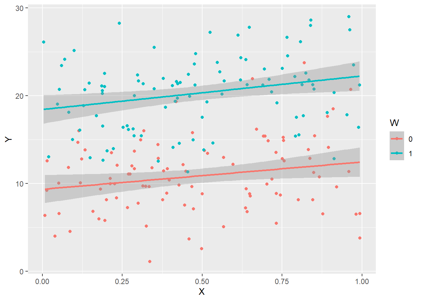

Association between the predictor of interest (X) and the outcome (Y) by the precision variable (W)

2.3.4 Adjusted and unadjusted regression models

• Unadjusted: \(E[Y|X] = \beta_0 + \beta_1*X\)
• Adjusted: \(E[Y|X] = \beta_0 + \beta_1*X + \beta_2*W\)

summary(lm(Y ~ X, data=precisiondata))

Fitting linear model: Y ~ X

Residuals

Min	1Q	Median	3Q	Max
-13.953	-4.6804	-0.76751	5.5132	13.526

	Estimate	Std. Error	t value	Pr(>|t|)
(Intercept)	13.8858	0.88218	15.7403	0.000000
X	3.4619	1.58179	2.1886	0.029796

Observations	Residual Std. Error	\(R^2\)	Adjusted \(R^2\)
200	6.2267	0.02362	0.018689

F-statistic: 4.78998 on 1 and 198 DF, pvalue: 0.0297956

summary(lm(Y ~ X + W, data=precisiondata))

Fitting linear model: Y ~ X + W

Residuals

Min	1Q	Median	3Q	Max
-9.24	-2.8797	0.34646	2.3857	11.717

	Estimate	Std. Error	t value	Pr(>|t|)
(Intercept)	9.1712	0.64172	14.2916	0.00000000
X	3.4659	1.02945	3.3667	0.00091453
W1	9.4252	0.57310	16.4460	0.00000000

Observations	Residual Std. Error	\(R^2\)	Adjusted \(R^2\)
200	4.0524	0.58854	0.58436

F-statistic: 140.89 on 2 and 197 DF, pvalue: < 2.22e-16

library(finalfit)

explanatory = c("X", "W")
dependent = "Y"

finalfit(.data = precisiondata, dependent, explanatory)

Dependent: Y		unit	value	Coefficient (univariable)	Coefficient (multivariable)
X	[0.0,1.0]	Mean (sd)	15.6 (6.3)	3.46 (0.34 to 6.58, p=0.030)	3.47 (1.44 to 5.50, p=0.001)
W	0	Mean (sd)	10.8 (4.1)	-	-
	1	Mean (sd)	20.3 (4.2)	9.42 (8.27 to 10.58, p<0.001)	9.43 (8.30 to 10.56, p<0.001)

3 Sampling Distributions

• The sampling distribution is the probability distribution of a statistic

  • e.g. the sampling distribution of the sample mean is \(N\left(\mu, \frac{\sigma^2}{n}\right)\)

• Most often we choose estimators that are asymptotically Normally distributed

  • For large \(n\), \(\hat{\theta} \sim N\left(\theta, \frac{V}{n} \right)\)

  • \(\hat{\theta}\) is our estimate of \(\theta\). The \(\hat{ }\) indicates it is an estimate.

  • Mean: \(\theta\)

• Variance: \(V\), which is related to the “average amount of statistical information” available from each observation

  • Often \(V\) depends on \(\theta\)

“Large” \(n\) depends on the distribution of the underlying data. If \(n\) is large enough, approximate Normality of \(\hat{\theta}\) will hold.

Calculating \(100 (1-\alpha)\%\) confidence intervals \(\left(\theta_L, \theta_U \right)\) with approximate Normality

• \(\theta_L = \hat{\theta} - Z_{1-\alpha/2} \sqrt{\frac{V}{n}}\)

• \(\theta_U = \hat{\theta} + Z_{1-\alpha/2} \sqrt{\frac{V}{n}}\)

• (estimate) \(\pm\) (crit val) \(\times\) (std err of estimate)

Can similarly calculate approximate two-sided \(p\)-values

• \(Z = \frac{\textrm{(estimate)} - \textrm{(hyp value)}}{\textrm{(std err of estimate)}}\)

4 Precision and Power/Sample Size

• What are the measures of (high) precision?

  • Estimators are less variable across studies, which is often measured by decreased standard error.

  • Narrower confidence intervals. Estimators are consistent with fewer hypotheses if the CIs are narrow.

  • Able to reject false hypotheses. Z statistic is higher when the alternative hypothesis is true.

• Translation into sample size

  • Based on the width of the confidence interval

  • Choose a sample size such that a 95% CI will not contain both the null and design alternative

  • If both \(\theta_0\) and \(\theta_1\) cannot be in the CI, we have discriminated between those hypotheses

• Based on statistical power

  • When the alternative is true, have a high probability of rejecting the null

  • In other words, minimize the type II error rate

• Statistical power: Quick review

  • Power is the probability of rejecting the null hypothesis when the alternative is true

  • Pr(reject \(H_0 | \theta = \theta_1\))

  • Most often \(\hat{\theta} \sim N\left(\theta, \frac{V}{n} \right)\) so that the test statistic \(Z = \frac{\hat{\theta} - \theta_0}{\sqrt{V/n}}\) wll follow a Normal distribution

  • Under \(H_0\), \(Z \sim N(0, 1)\) so we reject \(H_0\) if \(|Z| > Z_{1-\alpha/2}\)

  • Under \(H_1\), \(Z \sim N\left(\frac{\theta_1 - \theta_0}{\sqrt{V/n}}, 1\right)\)

• Power curves

  • The power function (power curve) is a function of the true value of \(\theta\)

  • We can compute power for every value of \(\theta\)

  • As \(\theta\) moves away from \(\theta_0\), power increases (for two-sided alternatives)

  • For any choice of desired power, there is always some \(\theta\) such that the study has that power

  • \(Pwr(\theta_0) = \alpha\), the type I error rate

mydiffs <- seq(-.8,.8,.05)

mypower <- vector("numeric", length(mydiffs))
mypower2 <- vector("numeric", length(mydiffs))

for(i in 1:length(mydiffs)){
   mypower[i] <- power.t.test(n=100, sd=1, delta=mydiffs[i])$power
   mypower2[i] <- power.t.test(n=100, sd=1.2, delta=mydiffs[i])$power
}

plot(mydiffs, mypower, xlab="True difference in means (theta)", ylab="Power", type="l", main="")
lines(mydiffs, mypower2, lty=2)
legend("top", c("sigma = 1.0","sigma = 1.2"), lty=1:2, inset=0.05)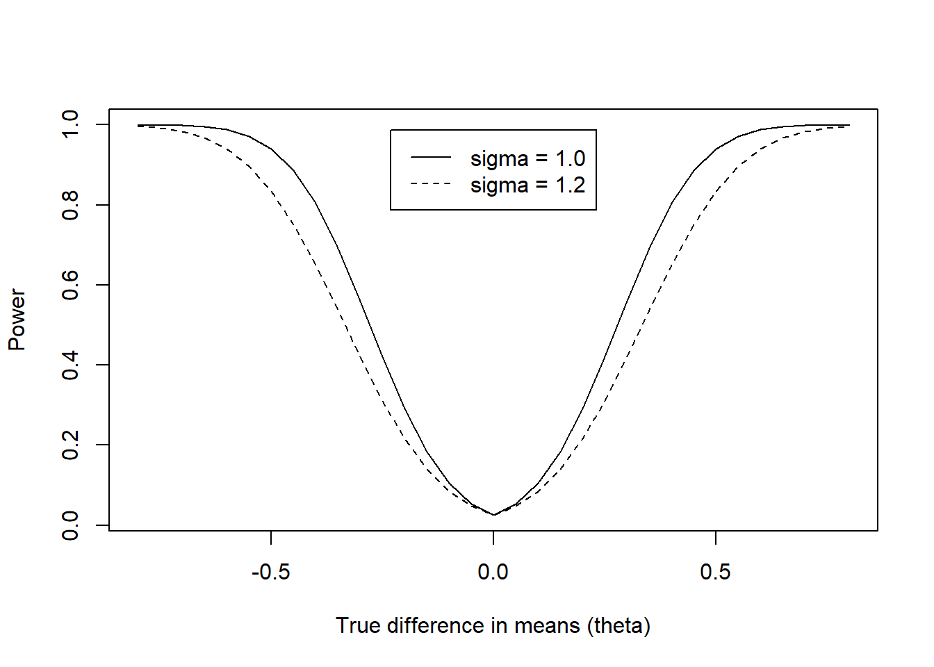

Power curves for a two-sample, equal variance, t-test; n=100

5 Precision and Standard Errors

• Standard errors are the key to precision

• Greater precision is achieved with smaller standard errors

• Standard errors are decreased by either decreasing \(V\) or increasing \(n\)

  • Typically: \(se(\hat{\theta}) = \sqrt{\frac{V}{n}}\)

  • Width of CI: \(2 \times (\textrm{crit value}) \times se(\hat{\theta})\)

  • Test statistic: \(Z = \frac{\hat{\theta} - \theta_0}{se(\hat{\theta})}\)

5.1 Example: One sample mean

• Observations are independent and identically distributed (iid)

  • \(\textrm{iid } Y_i \sim (\mu, \sigma^2), i = 1, \ldots, n\)

  • \(\theta = \mu\), \(\hat{\theta} = \frac{1}{n} \displaystyle \sum_{i=1}^n Y_i = \overline{Y}\)

  • \(V = \sigma^2\), \(se(\hat{\theta}) = \sqrt{\frac{\sigma^2}{n}}\)

• Note that we are not assuming a specific distribution for \(Y_i\), just that the distribution has a mean and variance

• We are assuming that \(n\) is large so asymptotic results are applicable

  • Then the distribution \(Y_i\) could be binary data, Poisson, exponential, normal, etc. and the results will hold

• There are ways to decrease \(V\) including…

  • Restrict sample by age, gender, etc.

  • Take repeated measures on each subject, summarize, and perform test on summary measures

  • Better ideas (this course)

    • Adjust for age and gender rather than restrict
    • Use all repeated observations and modeling correlation

5.2 Example: Two sample mean

• Difference of independent means

• Observations no longer identically distributed, just independent. Group 1 has a different mean and variance than group 2

  • \(\textrm{ind } Y_{ij} \sim (\mu_j, \sigma_j^2), j = 1, 2; i = 1, \ldots, n_j\)

  • \(n = n_1 + n_2\); \(r = n_1 / n_2\)

  • \(\theta = \mu_1 - \mu_2\), \(\hat{\theta} = \overline{Y}_1 - \overline{Y}_2\)

  • \(V = (r+1)(\frac{\sigma_1^2}{r} + \sigma_2^2)\)

  • \(se(\hat{\theta}) = \sqrt{\frac{V}{n}} = \sqrt{\frac{\sigma_1^2}{n_1} + \frac{\sigma_2^2}{n_2}}\)

5.3 Comments on the optimal ratio of sample sizes (\(r\))

• If we are constrained by the maximal sample size \(n = n_1 + n_2\)

  • Smallest \(V\) when \(r = \frac{n_1}{n_2} = \frac{\sigma_1}{\sigma_2}\)

  • In other words, smaller \(V\) if we sample more subjects from the more variable group

• If we are unconstrained by the maximal sample size, there is a point of diminishing returns

• Example: Case-control study where finding cases is difficult/expensive but finding controls is easy/cheap

  • Often quoted little benefit beyond \(r = 5\). That is, little benefit in having more than 5 times as many controls as cases

var.fn <- function(r, s1, s2) {
  (r + 1) * (s1^2/r + s2^2)
}

# Optimal sample size ratio for fixed sample size

n <- 100
s2 <- 10

plot(function(r) sqrt(var.fn(r, s1=s2, s2=s2) / n), 0, 20, ylim=c(1,6), xlim=c(0,25), ylab="Standard Error", xlab="Sample Size Ratio r = n1/n2")
plot(function(r) sqrt(var.fn(r, s1=2*s2, s2=s2) / n), 0, 20, add=TRUE, lty=2)
plot(function(r) sqrt(var.fn(r, s1=3*s2, s2=s2) / n), 0, 20, add=TRUE, lty=3)
text(20,4.7,"s1 = s2", pos=4)
text(20,5.1,"s1 = 2*s2", pos=4)
text(20,5.5,"s1 = 3*s2", pos=4)
points(c(1,2,3), sqrt(var.fn(c(1,2,3), s1=c(1,2,3)*s2, s2=s2)/ n), pch=2)
text(1, 1.8, "r = 1")
text(2, 2.8, "r = 2")
text(3, 3.8, "r = 3")

Optimal r for Fixed (n1 + n2). r = s1 / s2, the ratio of standard deviations in the two group.

n1 <- 200

plot(function(r) sqrt(var.fn(r, s1=s2, s2=s2) / (n1 + r*n1)), 0, 20, ylim=c(0.5,3), xlim=c(0,25), ylab="Standard Error", xlab="Sample Size Ratio r = n1/n2")
plot(function(r) sqrt(var.fn(r, s1=2*s2, s2=s2) / (n1 + r*n1)), 0, 20, add=TRUE, lty=2)
plot(function(r) sqrt(var.fn(r, s1=3*s2, s2=s2) / (n1 + r*n1)), 0, 20, add=TRUE, lty=3)

text(20,.7,"s1 = s2", pos=4)
text(20,.8,"s1 = 2*s2", pos=4)
text(20,.9,"s1 = 3*s2", pos=4)

Diminishing returns for r > 5. s1 and s2 are the standard deviations is group 1 and group 2, respectively. s1=s2 indicates the two groups have equal variablility. Other conditions represent the cases where the group we are oversampling has more variability.

5.4 Example: Paired means

• Difference of paired means

• No longer iid. Group 1 has a different mean and variance than group 2, and observations are paired (correlated)

  • \(Y_{ij} \sim (\mu_j, \sigma_j^2), j = 1, 2; i = 1, \ldots, n\)

  • \(corr(Y_{i1}, Y_{i2}) = \rho; corr(Y_{ij}, Y_{mk}) = 0 \textrm{ if } i \neq m\)

  • \(\theta = \mu_1 - \mu_2\), \(\hat{\theta} = \overline{Y}_1 - \overline{Y}_2\)

  • \(V = \sigma_1^2+ \sigma_2^2 - 2 \rho \sigma_1 \sigma_2\)

  • \(se(\hat{\theta}) = \sqrt{\frac{V}{n}}\)

• Precision gains are made when matched observations are positively correlated (\(\rho > 0\))

  • Usually the case, but possible exceptions

    • Sleep on successive nights

    • Intrauterine growth of litter-mates

5.5 Example: Clustered data

• Clustered data: Experiment where treatments/interventions are assigned based on the basis of “clusters”

  • Households

  • Schools

  • Clinics

  • Cities

• Mean of clustered data

  • \(Y_{ij} \sim (\mu, \sigma^2), i = 1, \ldots, n; j = 1, \ldots, m\)

• Up to \(n\) clusters, each of which have \(m\) subjects

  • \(corr(Y_{ij}, Y_{ik}) = \rho \textrm{ if } j \neq k\)

  • \(corr(Y_{ij}, Y_{mk}) = 0 \textrm{ if } i \neq m\)

• \(\theta = \mu\), \(\hat{\theta} = \frac{1}{nm} \displaystyle \sum_{i=1}^{n} \sum_{j=1}^m Y_{ij} = \overline{Y}\)

• \(V = \sigma^2 \left(\frac{1 + (m-1)\rho}{m} \right)\)

• \(se(\hat{\theta}) = \sqrt{\frac{V}{n}}\)

What is V if …

• \(\rho = 0\) (independent)

• \(m = 1\)

• \(m\) is large (e.g \(m = 1000\)) and \(\rho\) is 0, 1, or 0.01

• With clustered data, even small correlations can be very important to consider

  • Equal precision achieved with

Clusters (\(n\))	\(m\)	\(\rho\)	Total N
1000	1	0.01	1000
650	2	0.30	1300
550	2	0.10	1100
190	10	0.10	1900
109	10	0.01	1090
20	100	0.01	2000

• Always consider practical issues. Is it easier/cheaper to collect 1 observation on 1000 different subjects (\(n=1000\), \(m=1\)), or 100 observations on 20 different subjects (\(n=20\), \(m=100\))? These two designs have equal precision.

5.6 Example: Independent Odds Ratios

• Binary outcomes

• \(\textrm{ind } Y_{ij} \sim B(1, p_j), i = 1, \ldots, n_j; j = 1, 2\)

• \(n = n_1 + n_2; r = n_1 / n_2\)

• \(\theta = \textrm{log}\left(\frac{p_1/(1-p_1)}{p_2/(1-p_2)} \right)\); \(\hat{\theta} = \textrm{log}\left(\frac{\hat{p}_1/(1-\hat{p}_1)}{\hat{p}_2/(1-\hat{p}_2)} \right)\)

• \(\sigma^2_j = \frac{1}{p_j(1-p_j)} = \frac{1}{p_j(q_j)}\)

• \(V = (r+1)(\frac{\sigma_1^2}{r} + \sigma_2^2)\)

• \(se(\hat{\theta}) = \sqrt{\frac{V}{n}} = \sqrt{\frac{1}{n_1 p_1 q_1} + \frac{1}{n_2 p_2 q_2}}\)

• Notes on maximum precision

  • Max precision is achieved when the underlying odds are near 1 (proportions near 0.5)

  • If we were considering differences in proportions, the max precision is achieved when the underlying proportions are near 0 or 1

5.7 Example: Hazard Ratios

• Independent censored time to event outcomes

  • \((T_{ij}, \delta_{ij}), i = 1, \ldots, n_j; j = 1, 2\)

  • \(n = n_1 + n_2; r = n_1 / n_2\)

  • \(\theta = \textrm{log(HR)}\); \(\hat{\theta} = \hat{\beta}\) from proportional hazards (PH) regression

  • \(V = \frac{(r+1)(1/r+1)}{\textrm{Pr}(\delta_{ij} = 1)}\)

  • \(se(\hat{\theta}) = \sqrt{\frac{V}{n}} = \sqrt{\frac{(r+1)(1/r+1)}{d}}\)

• In the PH model, statistical information is roughly proportional to \(d\), the number of observed events

  • Papers always report the number of events

  • Study design must consider how long it will take to observe events (e.g. deaths) starting from randomization

5.8 Example: Linear Regression

• Independent continuous outcomes associated with covariates

  • \(\textrm{ind } Y_i | X_i ~ \sim(\beta_0 + \beta_1 X_i, \sigma^2_{Y|X}), i = 1, \ldots, n\)

  • \(\theta = \beta_1, \hat{\theta} = \hat{\beta_1}\) from LS regression

  • \(V = \frac{\sigma^2_{Y|X}}{\textrm{Var}(X)}\)

  • \(se(\hat{\theta}) = \sqrt{\frac{\hat{\sigma}^2_{Y|X}}{n \hat{\textrm{Var}}(X)}}\)

• Precision tends to increases as the predictor (\(X\)) is measured over a wider range

• Precision also related to the within group variance \(\sigma^2_{Y|X}\)

  • What happens to the formulas when \(X\) is a binary variable? See two sample mean

6 Summary and Concluding Comments

• Options for increasing precision

  • Increase sample size

  • Decrease \(V\)

  • (Decrease confidence level)

• Criteria for precision

  • Standard error

  • Width of confidence intervals

  • Statistical power

• Select a suitable, scientifically meaningful alternative

  • With proper precision, can distinguish between minor and meaningful effects

• Select desired power

• Sample size calculation: The number of sampling units needed to obtain the desired precision

  • Level of significance \(\alpha\) when \(\theta = \theta_0\)

  • Power \(\beta\) when \(\theta = \theta_1\)

  • Variability \(V\) within one sampling unit

  • \(n = \frac{(z_{1-\alpha/2} + z_{1-\beta})^2 \times V}{(\theta_1 - \theta_0)^2}\)

• When sample size is constrained (the usual case) either

  • Compute power to detect a specified alternative

    • \(1 - \beta = \phi \left(\frac{(\theta_1-\theta_0)}{\sqrt{V/n}} - z_{1-\alpha/2} \right)\)

    • \(\phi\) is the standard Normal cdf function

    • In STATA, use normprob for the \(\phi\) function

  • Compute alternative that can be detected with high power

    • \(\theta_1 = \theta_0 + (z_{1-\alpha/2} + z_{1-\beta}) \sqrt{V/n}\)

6.1 General Comments

• Sample size required behaves like the square of the width of the CI. To cut the width of the CI in half, need to quadruple the sample size.

• Positively correlated observations within the same group provide less precision than the same number of independent observations

• Positively correlated observations across groups provide more precision

• What power do you use?

  • Most popular is 80% (too low) or 90%

  • Key is to be able to discriminate between scientifically meaningful hypotheses